Coincidentally, sometime after moving to Tampa in 1995, I found that a very similar effort was carried out at Microsoft Lab as part of a project titled as "Surface Reconstruction", which was used for developing games. Very recently, the similar technology is being used for 3D printing (a very promising emerging technology), as a 3D model can be represented by a series of triangular shapes before making it to a real part through 3D printer.
Unfortunately, the algorithm of mesh generation or surface reconstruction (no matter how it is called) that Dr. Parviz Navi and I developed almost 20 years ago has never been officially published. What happened was we wanted to publish it on an academic journal. I wrote the majority of a draft describing the algorithm, and waiting for Dr. Navi to write the first section as an introduction. However, he never finished this section by any reasons. I would like to put the original draft as my blog for the memory of an unforgettable period of my time living in Switzerland.
(some notations are messed up due to HTML being not able to represent Greek letters.)
2 DESCRIPTIONS
The method of the triangle mesh
generation proposed in this article will be described here. Section 2.1 will
give the definitions and observations made about triangle generation. Next we
will be discussing about the triangulation. Finally the optimization methods
that we have been using is introduced.
2.1 Definitions and Observations
Throughout this paper, we will
use the terminology as exterior and interior boundaries, fixed points, movable
points and connections. Their definitions are given as follows.
Exterior boundary: a line
that outlines the outermost shape of a domain.
Interior boundary: a line
that outlines a void inside a domain.
Fixed points: points used to
define the boundary of a domain to be meshed. The boundary can be exterior or
in interior.
Movable points: points
inside a domain. The position of the movable points will be shifted up to the
optimization criterion.
Connection: a straight line
connecting one point to the other. Connections are grouped as fixed and
non-fixed connections.
Fixed connection: a
connection between two fixed points. The fixed connections online either an
exterior or interior boundary.
Non-fixed connection: a
connection between a fixed point and a non-fixed point, or between two
non-fixed points.
Figure 2.1 shows graphically the
fixed, movable points and connections.

Fig. 2.1 Definition of fixed, movable points and
connections.

Fig. 2.2 Schematic representation of relationship
among the positions of movable points (Sp),
their connections (Sc)
and corresponding meshes.
As it is shown in Figure 2.2, a
set of different possible positions and their connections will result in
different meshes. Usually, these meshes do not meet with the precision
requirement of calculation without undergoing an optimization process. The optimization
process will improve the performance of the mesh. Hence, the aim becomes to find an optimized
mesh from those with different values of Sp and Sc.
The relationship of the positions of the movable points, their connections in
terms of the mesh performance is shown in Figure 2.3. It's possible to achieve this aim by
following two different passages, (1) altering the value of Sp,
which means to shift the positions of the movable points, and (2) changing the
value of Sc,
which means to rearrange the connections of the movable points. The
optimization methods that we use will be described in Section 2.3.

Fig.2.3 Schematic
representation of mesh performance in terms of
position of movable
points (Sp),
their connections (Sc).
2.2 Triangulation
Before the triangulation starts,
the fixed connections (see the definition of the fixed connection in Section
2.1) should be established. The fixed
connections online the boundary of a domain. The boundary can be either
exterior or interior. Next, a simple
triangulation method is used. It starts from connecting one point to the other,
no matter it is a fixed or movable point.
Figure 2.4(a) shows the possible connections for the point 1 (1-6, 1-3
and 1-5) and the connection for point 2 (2-5).
When connecting one point to the
other, the following two criteria must be checked:
- No connection has been existed for the two points to be connected. This can be further explained by the aid of the example shown in Figure 2.4(a). For instance, before the connection between the point 1 and 6 is established, the program should check if there is already a connection between these two points. If it's so, then the connection should be aborted.
- A connection to be established should not intersect with any existing connections. For example, a connection from point 4 to point 5 in Figure 2.4(a) should not be allowed, since it will intersect with the connection 1-3.
After the process of the
connection goes through all points, the triangulation is completed. An example
of the final triangulation is shown in Figure 2.4(b).

Fig. 2.4 Triangulation – connecting one point with the
other.
2.3 Optimization of Triangles
As mentioned above, we optimize a
triangular mesh by rearranging the non-fix connections and by changing the
movable points' position. We note that
each movable point, in the case of triangular mesh, is surrounded by a polygon
(a triangle is also treated as a polygon.).
There are two types of polygon, concave and convex, as shown in Figure
2.5. Our optimization algorithm needs to
know if a polygon is concave or convex.
It is found that in the case of a concave polygon (Figure 2.5(b)), the
area constructed by the points 1-2-3 is negative due to clock-wise counting of
the points. While, for a convex polygon, the same area calculated by connecting
the points 1-2-3 is positive. Therefore, to determine whether a polygon is a
concave or convex, successive areas constructed by the points 1-2-3, 2-3-4,
etc. (Figure 2.5) are calculated. If an area is negative, then, the polygon is
concave. After knowing the type of the polygon surrounding each movable point,
we are about to discussing the proposed optimization as follows.

Fig. 2.5 Definition of convex and concave
polygon: (a) Convex; (b) Concave.
2.3.1 Changing the movable points
This optimization is performed
for both convex and concave polygons. For a convex polygon, the point inside
the polygon will simply be moved to the centroid of the polygon. While for a
concave polygon, a two-step process will be followed. We will use an example shown in Figure 2.6 to
explain the two-step process. The
initial triangular elements and concave polygon are shown in Figure 2.6(a). The
movable point is labeled by the letter P.
Step 1: The two
connections D-E and D-C (connecting to the vertex D of a concave polygon, Figure 2.6) will
be extended. In the example shown in
Figure 2.6, the extension of the two connections will insect with other
connections of the polygon. The intersection points are I and J, in Figure
2.6. The extension process results in a
convex polygon indicated by A-J-D-I-F.
Step 2: The movable point
P will be moved to the centroid of
the resulting polygon A-J-D-F, same
as we do for other convex polygons. The
final triangular elements are shown in Figure 2.6(b).
It is found that the point P can not be placed outside the polygon A-J-D-I-F, resulted from the extension
of the connections D-E and D-C.
Otherwise, one of the connections between the point P and the points A, B, C, D,
E, F will intersect with other connections.
For instance, if the point P is placed inside the polygon B-C-D-J, then the connection P-E will intersect with the connection D-C.
As a result that the point P must be inside the convex polygon A-J-D-I-F, question becomes where this
point should be placed. We place it at the centroid of the convex polygon, as
mentioned in the step 2.

Fig. 2.6 Replacing the movable point P: (a) initial position of the
point P and triangular elements; (b) final
position of the point P and
triangular elements.
2.3.2 Rearranging the non-fix connections
Rearranging the non-fixed
connections are performed only for the convex polygon. Figure 2.7 gives an
example of this rearrangement. Basing on
the direct judgement, we know that the connection A-C has to be changed to B-D,
shown in Figure 2.7. This is because the
triangle ADB and DCB (Figure 2.7 (b)) is closer to the equilateral triangle than ADC and ACB (Figure 2.7(a)).
However, the direct judgement cannot be coded into a computer program.
Hence, for this respect, a more general criterion has been formulated.

Fig. 2.7 Rearranging the movable point's connection.
It is well know that every
triangle is well defined by three internal angles, a, b and g. As a result, a vector can be constructed in
the space of a,
b
and g
as  = {a, b, g}. Note that a + b + g = 180o, which represents a plane
intersecting with a,
b
and g
axis at 180o, shown in Figure 2.8. Any triangle will be a point on
the plane, pointed by the corresponding vector of its internal angles.
The point on the plane for an equilateral triangle will be pointed by
the vector
= {a, b, g}. Note that a + b + g = 180o, which represents a plane
intersecting with a,
b
and g
axis at 180o, shown in Figure 2.8. Any triangle will be a point on
the plane, pointed by the corresponding vector of its internal angles.
The point on the plane for an equilateral triangle will be pointed by
the vector  ={60, 60, 60}. It can
be easily approved that (={60, 60, 60}) is perpendicular to the plane. In other word,
the magnitude of for the equilateral triangle will be the minimum among the
magnitudes of all .
={60, 60, 60}. It can
be easily approved that (={60, 60, 60}) is perpendicular to the plane. In other word,
the magnitude of for the equilateral triangle will be the minimum among the
magnitudes of all .

Fig. 2.8 Plane representing any triangle in the space
defined by the internal angles a, b and g of
triangles.
Hence, to determine if a
non-fixed connection should be rearranged, the sum of the magnitudes is
calculated forfor the two adjacent triangles. In the case shown in Figure 2.7 (a), the
magnitudes of the vectors for triangles ACB
and ADC will be calculated. The sum
of the two magnitudes is made. Then, this sum is compared with that for the
triangles ADB and BDC, from Figure 2.7(b). Since the latter is less than the former, the
connection A-C (Figure 2.7(a)) will
be replaced by B-D (Figure 2.7(b)).
The optimization process of
changing the movable points and rearranging the non-fixed connections is
performed alternatively. This process is also repeated for a few times. Our
experience shows that after several iterations of the optimization, the shape of
triangular elements will be improved greatly and stabilized. The numbers of the movable points changed and
of the non-fixed connections rearranged are recorded during the iterations of
the optimization process. When the numbers are smaller than a given value, then
the iteration can be stopped. Examples
from above-described triangulation and optimization will be shown in the next
section.
3 EXAMPLES AND DISCUSSIONS
After giving the triangulation
and its optimization algorithms in the last section, we are now in the position
to show the results from their applications.
Three examples will be illustrated in this section to show the
workability of our triangulation method and the efficiency of the optimization
algorithm. A brief discussion will be followed for each example as well.
3.1 Example 1 – a structure of particle reinforced materials
Domains used in this example are
composed of two different materials: matrix and irregular grains. The grains usually have different properties
from those of the matrix, for instance, stiffer than the matrix. As a result, the triangles corresponding to
the matrix and grains must be distinguished, before the finite element
calculation is performed for the composite.
As the first step to mesh the composite, we generated a set of fixed
points for the outer boundary of the composite specimen and for the boundary of
grains, as well as a set of the movable points inside the doma0ins. The result after the operation of the first
step is shown in Figure 3.1(a).
Subsequently, the fixed connections are established within the fixed
points. Then, both fixed and movable
points are connected each other by the method described in Section 2.2. The initial triangles are shown in Figure
3.1(b). Finally, the resulted triangular
mesh after an initial optimization and third iteration are respectively shown
in Figure 3.1(c) and (d).
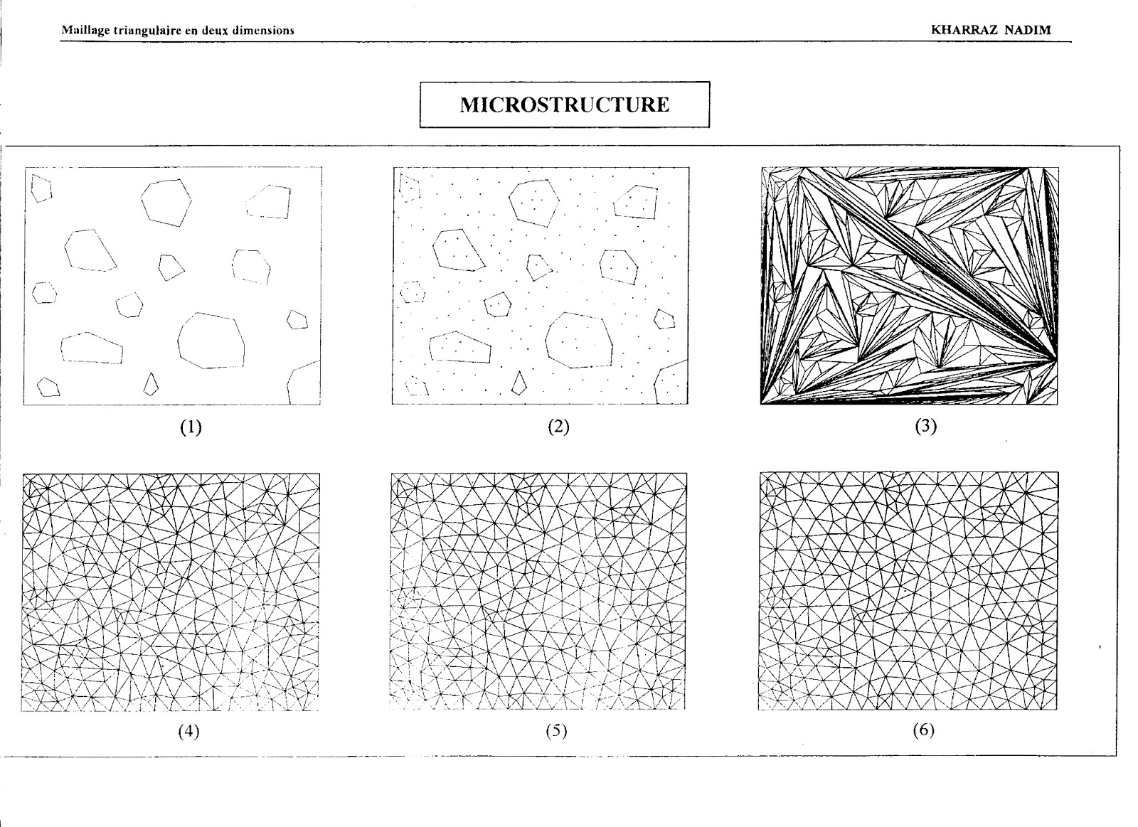
Fig. 3.1 Example of triangular mesh generation for a composite.
(a) Fixed and movable points, as well as fixed connections.
(b) Initial triangular elements after connecting each points.
(c) Triangles after first iteration of optimization.
(d) Triangles after third iteration of optimization.
(a) Fixed and movable points, as well as fixed connections.
(b) Initial triangular elements after connecting each points.
(c) Triangles after first iteration of optimization.
(d) Triangles after third iteration of optimization.
3.2 Example 2 – a structure of fiber reinforced materials
As shown in the last example, the mesh generation method
that we proposed in this article works for any case. It is especially powerful
tool for the study of composites. Here
another example of composite – fiber reinforced materials is given. This material is composed of a matrix and
fibers, which are embedded in the matrix with a regular pattern. Examples of fiber reinforcement materials can
be the natural wood material or synthesis fiber reinforced plastic.
Figure 3.2(a) shows the results after the generation of the
fixed, movable points and the fixed connections. The initial triangular
elements are given in Figure 3.2(b). The
results corresponding to the first and final (third) iterations of optimization
are demonstrated in Figure 3.2(c) and (d) respectively.

Fig. 3.2 Example of triangular mesh generation for a
fiber reinforced material.
(a) Fixed and movable
points, as well as fixed connections.
(b) Initial
triangular elements after connecting each points.
(c) Triangles after
first iteration of optimization.
(d) Triangles after
third iteration of optimization.
3.3 Example 3– Swiss map
The last example given in this
paper is the triangular mesh for the map of Switzerland, where our university
is from. The outline of the Swiss map is quite irregular. Same as the previous two examples, we give
the fixed, movable points and the fixed connections in Figure 3.3(a). Note that there is inland lake (named Lake
Neuchatel) close to the left frontier of Switzerland. The initial triangular elements, elements
after the first and third (final) iterations of the optimization are
illustrated in Figure 3.3(b), (c) and (d) respectively.

Fig. 3.2 Example of triangular mesh generation for
Swiss map.
(a) Fixed and movable
points, as well as fixed connections.
(b) Initial
triangular elements after connecting each points.
(c) Triangles after
first iteration of optimization.
(d) Triangles after
third iteration of optimization.
4 CONCLUSIONS
In this paper, we have presented
a method of triangular mesh generation and algorithms to optimize the resulted
triangles. The method is based on the
concepts of fixed and movable points, as well as connections between the
points. A connection is further
distinguished into the fixed and non-fixed one.
The fixed connections form the boundary for a domain to be meshed. The optimization process works on moving the
movable points and on rearranging the non-fixed connections.
The studies on the proposed
method and the algorithms show that they have the following characteristics and
advantages comparing other methods.